• To handle overlapping classes
• Linearity condition remains
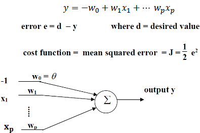
  • Linear boundary
• No hard limiter
  • Linear neuron
• Cost function changed to error, $J$
  • Half doesn’t matter for error
    • Disappears when differentiating

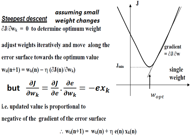
• Cost’ w.r.t to weights

  $$\frac{\partial\mathfrak{E}(w)}{\partial w}=e(n)\frac{\partial e(n)}{\partial w}$$

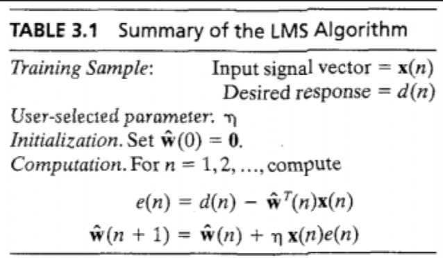
• Calculate error, define delta

  $$e(n)=d(n)-x^T(n)\cdot w(n)$$
  $$\frac{\partial e(n)}{\partial w(n)}=-x(n)$$
  $$\frac{\partial \mathfrak{E}(w)}{\partial w(n)}=-x(n)\cdot e(n)$$

• Gradient vector

  • $g=\nabla\mathfrak{E}(w)$
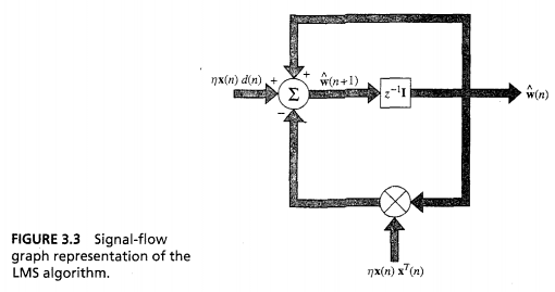
  • Estimate via: $\hat{g}(n)=-x(n)\cdot e(n)$ $\hat{w}(n+1)=\hat{w}(n)+\eta \cdot x(n) \cdot e(n)$

• Above is a feedforward loop around weight vector, $\hat{w}$

  • Behaves like low-pass filter
    • Pass low frequency components of error signal
  • Average time constant of filtering action inversely proportional to learning-rate
    • Small value progresses algorithm slowly
      • Remembers more
      • Inverse of learning rate is measure of memory of LMS algorithm

• $\hat{w}$ because it’s an estimate of the weight vector that would result from steepest descent

  • Steepest descent follows well-defined trajectory through weight space for a given learning rate
  • LMS traces random trajectory
  • Stochastic gradient algorithm
  • Requires no knowledge of environmental statistics

Analysis

• Convergence behaviour dependent on statistics of input vector and learning rate
  • Another way is that for a given dataset, the learning rate is critical
• Convergence of the mean
  • $E[\hat{w}(n)]\rightarrow w_0 \text{ as } n\rightarrow \infty$
  • Converges to Wiener solution
  • Not helpful
• Convergence in the mean square
  • $E[e^2(n)]\rightarrow \text{constant, as }n\rightarrow\infty$
• Convergence in the mean square implies convergence in the mean
  • Not necessarily converse

Advantages

• Simple
• Model independent
  • Robust
• Optimal in accordance with $H^\infty$, minimax criterion
  • If you do not know what you are up against, plan for the worst and optimise
• Was considered an instantaneous approximation of gradient-descent

Disadvantages

• Slow rate of convergence
• Sensitivity to variation in eigenstructure of input
• Typically requires iterations of 10 x dimensionality of the input space
  • Worse with high-d input spaces
• Use steepest descent
• Partial derivatives
• Can be solved by matrix inversion
• Stochastic
  • Random progress
  • Will overall improve

Where

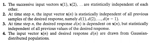
Independence Theory